Service Reports
The reports provided in the Reporting application section present the data collected by the Central Server®. If Service reports are used for this purpose, the way they are displayed is based explicitly on a Service that has been defined in the Master Data module.
This means that the Service report only contains the Data Sources and Locations that are part of the underlying Service. The Service report also takes account of the Service Times, Down Times, and Excluded Measurements that were defined for the underlying Service.
You can find a detailed description of Services here.

Only users with the Service Report Management Open privilege can access Service reports.
Multitenancy
Service reports are created in the context of the Customer currently selected. Standard users can only see Service reports for the Customer they are associated with.
System users can freely select Customers. After selecting a Customer using the Customer Switch, work carried out by the System User is performed in the context of that Customer. New reports created by System Users are then associated with the selected Customer for use by that Customer's users.
Caution: The System context does not support any Service reports. If the System context [System] is selected under the Customer Switch, the following message will appear:

Menu
The Service Reports overview contains the following menu items:
 Refresh
This menu item refreshes the list of Service reports. The table's status bar shows the time stamp of the last refresh.
Create
This menu item creates a new Service report.
User
This menu item is only available to users with the Service Report Create / Edit
privilege.
Rename
Every newly created report is given a name and description for the purposes of unique identification.
These parameters can be
modified later using this menu item.
User
This menu item is only available to users with the Service Report Create / Edit
privilege.
Remove
If a Service report is no longer required, it can be removed from the System using this menu item.
User
This menu item is only available to users with the Service Report Delete privilege.
Creating Service Reports
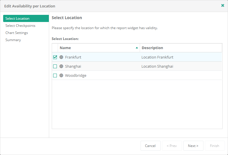
There are two options available to you when creating Service Reports. Option one creates an empty report (Create - Empty Service Report). Option two creates a report that contains important graphs, diagrams, and tables (Create - Prefilled Service Report). In both cases you must first select a Service on which the report is based. A Service report can only use one Service in each case.
To generate a Service report, you must first select a Service on which the report is based. A Service report can only use one Service in each case.
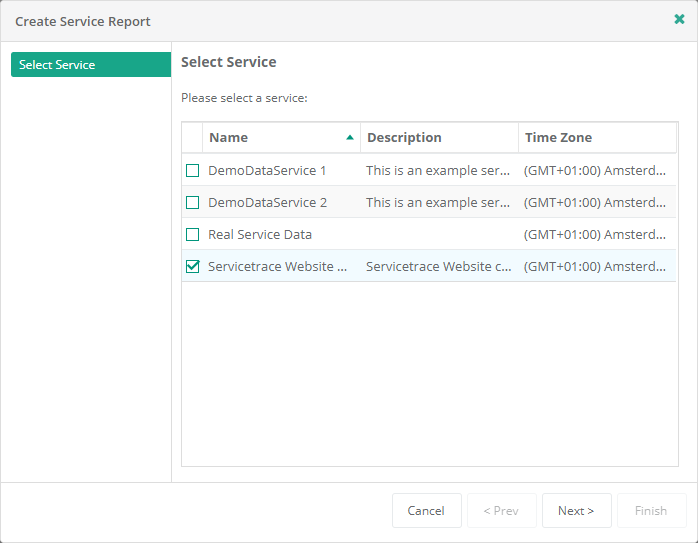
In the Service you define which Data Sources from which Locations should go into the report. You also stipulate whether and which Service Times and Down Times should be taken into account there. You can thus represent an IT service provided or used by you in the Central Server system. If you have not created any Services yet, first switch to the Master Data web app and create at least one Service in the Services section in order to be able to use Service reports. You can find a detailed description of Services here.
Once a Service has been selected, you are able to incorporate individual widgets or categories of widgets into the Service report. The choice of widgets depends on the content of the Service (Locations and Data Sources).

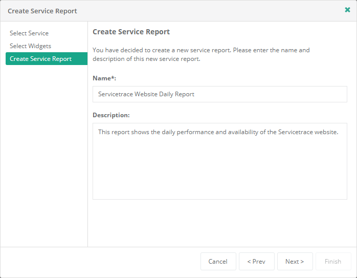
Now enter the name of the new Service report. At this point you can also save a more detailed description of the report. This is typically displayed in all selection menus and makes it easier to identify the report later.
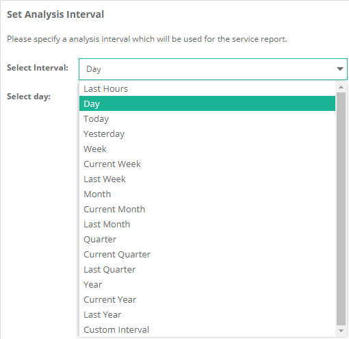
In the following step you define which period the report should display when it is opened. You can choose either a static or a dynamic period. A static period relates to a particular date such as October 3, 2014. A report with this static time configuration always displays the data from October 3, 2014, for example, when opened. For a dynamic period, the report is automatically adjusted for the point in time when the report is accessed. A report with a dynamic time configuration can be set to always display data from the last week, for example. Predefined time periods can be adjusted in opened reports. Any time range of interest can therefore be looked at without having to specially create a new report for it.

The following time ranges are available:
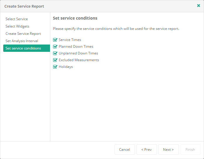
Finally you decide whether the Service report should take account of all the parameters defined in the Service, such as Service Times or Planned Down Times. In this respect it is important whether the report should provide evidence of compliance with Service Level Agreements (SLAs), or whether it will be used for technical analyses. If the report is expected to provide evidence of compliance with SLAs, all the parameters defined in the Service should be included in the report. If these parameters are not taken into account, the reports shows all the measurement data collected without exception and hence a comprehensive portrayal of the availability and performance of an IT Service.
The report creation process ends with an overview page. Click "Finish" to create the report with the parameters shown, or
navigate using "Prev" and "Next" to
modify the parameters.
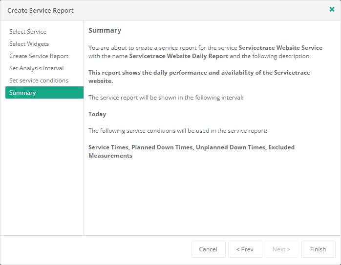
Clicking "Finish" automatically opens the report that has just been created.
Using Service Reports
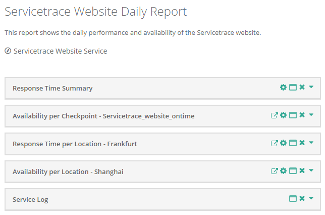
In the Service Reports section you can see a list of all the Service reports for the Customer selected. To open a report, please click on its name field.

The report itself is divided into different sections. The middle section shows the graphs, diagrams, and tables used to show measurement data. The section on the right lists the settings for the report and provides menu items for adjusting the report:
Menu
Refresh Data
Updates the Service report currently open. Only the graphs, diagrams, and tables that are open are refreshed. Any adjustments made to the report, even if they have not been saved, remain as they are. The time of the last refresh is specified in the individual widgets at the lower right.
 Settings
The settings are used to adjust the time range shown by the report, as well as to switch conditions defined by the Service on and off.
 Save
Save
If changes have been made to the report, such as adding more graphs or adjusting the time range shown, then these are initially only temporary for the current view. If the changes are intended to be adopted permanently and to apply the next time that the report is accessed, please save these using "Save".
 Save As...
If you want to retain an adjusted report as a separate report independently of the original, then the "Save As..." function can be used to create a new Service report very simply. Just give a new name and a new description, if required, to the new Service report and confirm with OK.
 Reload Report
If you want to load the report as it is filed in the System and discard any adjustments made to the report, use the Reload Report function. If changes have been made to the Data Sources contained in the Service since the report was last accessed, these are taken into account during the Reload Report process, which is not the case when using the "Refresh Data" function.
 Collapse All
Every widget contained in the report can be individually expanded or collapsed. This enables optimal use to be made of the space available and optimizes the time taken to load and display the relevant content. Use Collapse All to close all widgets at once to make space.
 Expand All
Every widget contained in the report can be individually expanded or collapsed. Use Expand All to open all widgets at once.
Settings
When a report is opened, this is loaded based on the settings saved. These are displayed on the right. The "Analysis Interval" shows the period under consideration currently selected. Service Conditions indicate the parameters that the report is currently taking into account for the underlying Service. Enabled Service Conditions are displayed in color, disabled ones are grayed out.

So that the Reporting function can be used as widely as possible, the predefined settings can be adjusted at any time. If, for example, you notice when looking at a daily report that response times have worsened, then you can simply expand the period under consideration to the whole week in order to determine exactly when performance started to deteriorate. Use the Report Settings to make such an adjustment. To open them, click on the cog wheel button in the Report Properties menu:
Changes to the settings of a report only relate to the current display and do not change the saved report. The adjusted settings are only permanently adopted within the report when you save them using "Save".
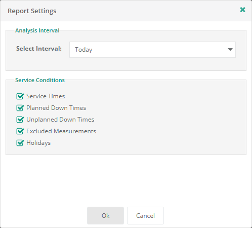
Settings - Analysis Interval
This setting defines the period contained in the report. If this does not involve an automatically determined, dynamic time range, e.g. "last week" or "last month", you can define a fixed time range at this point.
Settings - Service Conditions
This setting stipulates whether the parameters defined in the Service (Service Times, Down Times, Holidays and Excluded Measurements) are taken into account. When Service Times are enabled, only measurement data is taken into account that fall within the Service times stored within the Service. When Planned Down Times, Unplanned Down Times, Excluded Measurements or Holidays are enabled, measurement data within these periods are not taken into account in the report. Planned and Unplanned Down Times relate here to the measurement data for the entire Service, whereas Holidays and Excluded Measurements relate to measurement data for particular Locations. Disable all Service Conditions for a complete picture of the measurement data collected without exceptions. When doing so, watch out for entries in the Service Log, which may already contain references to analyses made regarding the data collected.
Confirm all the adjustments with OK.
Calendar
The calendar view of a report lists the parameters defined in the Service in increasing order in terms of time (Down Times, Excluded Measurements, and Holidays).
Service parameters are only taken into account if they are enabled in the Report Settings and lie within the period under consideration selected. If the unmodified 24x7 Default Service Time applies in the Location being looked at, this is not listed separately.
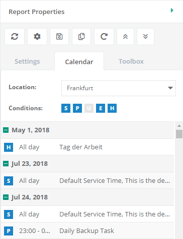
All times specified are automatically converted into the time zone of the user who is logged in. This ensures they are as easy to understand as possible. Please bear in mind that only the Down Times, Excluded Measurements, and Holidays of the Location selected can be displayed simultaneously. If you would like to look at the corresponding information for another Location, select this using the drop-down Location menu.
If the time range displayed contains several days with a lot of entries, you can get a better overview by using the minus sign to simply collapse the days that are not of immediate interest.
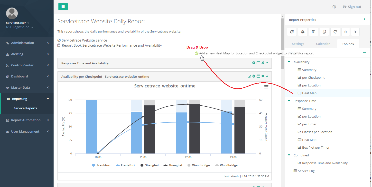
Toolbox
The Toolbox contains all the elements that can be placed in the Service Reports. These include various graphs, diagrams, and tables used to display the measurement data collected, which are known as widgets. You will also find the individual measurement points and Data Sources here, as well as different measurement Locations.
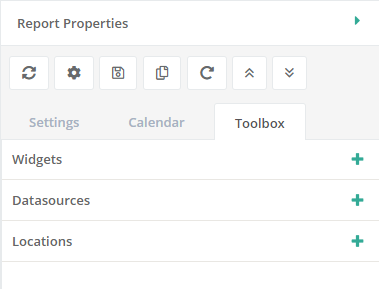
Select the toolbox section required by clicking on its plus button. The section is shown and you can place the elements it contains into the Service Report using drag and drop.
User
This function is only available to users with the Service Report Create / Edit
privilege.
Toolbox - Widgets
The display elements available are thematically arranged according to availability, response time, and additional information.
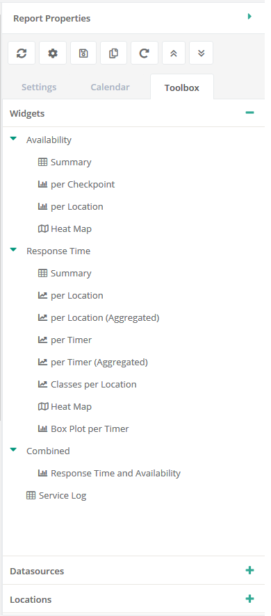
If you have created a new report using Create - Empty Service Report, you should initially populate this with widgets in the middle section. Further details about the individual widgets and their contents can be found here.
Toolbox - Data Sources
This toolbox section displays all the Data Sources that the Service underlying the report contains.

You can specifically populate individual widgets with particular Data Sources here. You can also integrate Data Sources newly added to the Service in existing widgets. Use drag and drop to drag the required Data Source to the corresponding widget in the report.
Toolbox - Locations
This toolbox section displays all the Locations that the Service underlying the report contains.

You can add other Locations here to widgets that break down your measurement data by Location. This applies in particular if Locations have recently been added to the Service and are intended to be integrated in widgets that already exist. Use drag and drop to drag the required Location to the corresponding widget in the report.
Widgets
To display the measurement data collected, the Reporting function uses individual widgets. A report can contain any number of widgets. Every widget can also be individually configured using its window controls.
Menu
 Settings
Apart from the Service Log, all widgets have their own configuration. This can be adjusted at any time using the settings. Depending on which type of data a widget displays, you can therefore define which Data Sources should be included in it from which Locations. For the exact description of the configuration, please read the section relating to the corresponding widget type.
User
This menu item is only available to users with the Service Report Create / Edit
privilege.
 Maximize
The Maximize button can be used to open a widget from the report as a separate window. You can thus make use of all the available space on the screen, for example to look at a graph in detail. The new window uses the same tab in the browser and overlays the Service report. The Service report itself is only accessible again once the maximized view of the widget has been closed using its Close button.
 Remove
If you want to remove a widget from the current report view, click on the Remove button. This change only becomes permanent if you use the Save button in the report settings. Otherwise the removed widget can be retrieved by opening the report again on the summary page or by using the Reload Report function.

 Close / Open
Certain preconfigured widgets may be expected to be a fixed part of a report. However, these should only load and display data if a specific detailed analysis is involved. Otherwise they should neither be taking up space nor delaying the construction of the report. In this case, individual widgets can be collapsed using the Close button. If, after a widget has been collapsed, the report is saved using Save, then the window will also be closed when the report initially loads. If the data it contains is then expected to be loaded and displayed, this can be done quickly and simply using the Open button – without any additional configuration.
 Export
  Download CSV
Click the "Download CSV" button to download the chart data that is presently being displayed. CSV is the file format.
Export  Generate Export URL
Servicetrace Reporting provides an interface for the usage of measurement data with external applications. This interface is implemented as a RESTful WebService. That means that Reporting data can be retrieved through a certain URL.
The URL consists of a base address (containing protocol, domain and port) completed with retrieval information (containing the widget to be exported, Customer, Service, time interval and several more). The password at the end of the expression (marked red in the image below) must be replaced with the actual password to be used. Thus the Export URL generated by pressing the button Export is only an example pattern. To retrieve the data no report must be created before. Detailed information regarding the generation of Export URLs can be found here.

The data is returned in CSV format with the vertical bar | as separator. For Availability per Checkpoint, Availability per
Location, Response Time per Location and
Response Timer per Timer the following data is exported:
Customer|service|Location|Station|datasource|workflow|date|value|hit
The timestamp of exported values use an accuracy of one second. This is also the accuracy of the values saved in the data base. The tool tips of the aggregation intervals in Response Time charts show times with an accuracy of one second as well. However, the aggregation intervals are computed with an accuracy of milliseconds. This may lead to deviations of at most one second when comparing the aggregated values of a chart to the export interface's values.
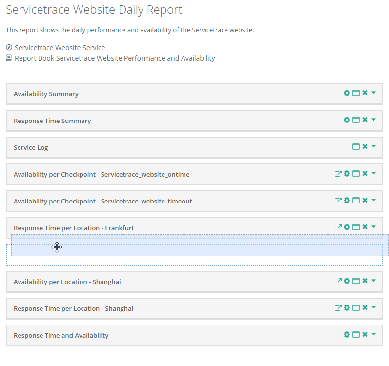
Placing widgets in the report
Each widget can be positioned anywhere in the report. In order to adjust the position of a widget, it is recommended to first collapse all windows using the Collapse All button. Then drag the relevant window to the new position using drag and drop. In order to save the changes permanently, finish the action with the Save button. If you have previously collapsed windows, do not forget to open these again before saving!
Widget types
Availability Summary
The "Availability Summary" widget is a list in table form of availabilities that have been collected. To determine availability, checkpoints are set up in the Workflows. The name of the checkpoint is given first accordingly. As measurements may have been taken from different Locations, the Location is also specified. After that, the availability value calculated is specified, as well as the number of measurements carried out and how many of them were successful or not successful. An average runtime is also given as additional information. This is the average of the period in seconds from the start of the Workflow until the checkpoint is reached. This period is only ascertained for checkpoints that have been measured successfully. The last row Overall Average shows the arithmetic average of all values shown in the respective column of the widget.
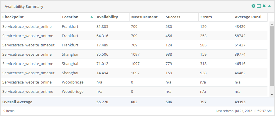
You can also hide the individual columns as required. As an option, you can additionally show to which System and which Application from the Master Data the checkpoint belongs.

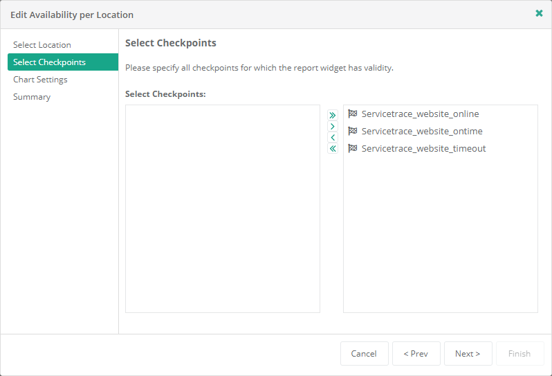
The settings of this widget can be used to specify which checkpoints should be included. It is also possible to define for which Locations the availability of these checkpoints should be listed.
User
This menu item is only available to users with the Service Report Create / Edit
privilege.
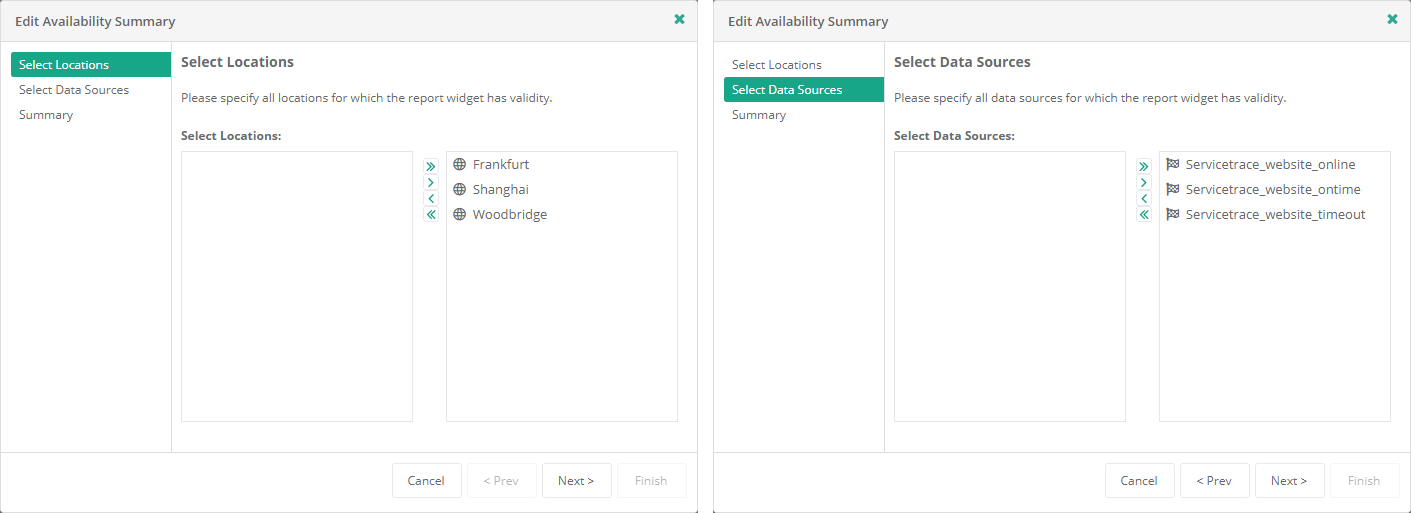
It is therefore possible to either display all the information in one window, or to pool all the checkpoints for one Location or all the Locations for one checkpoint in a single window.
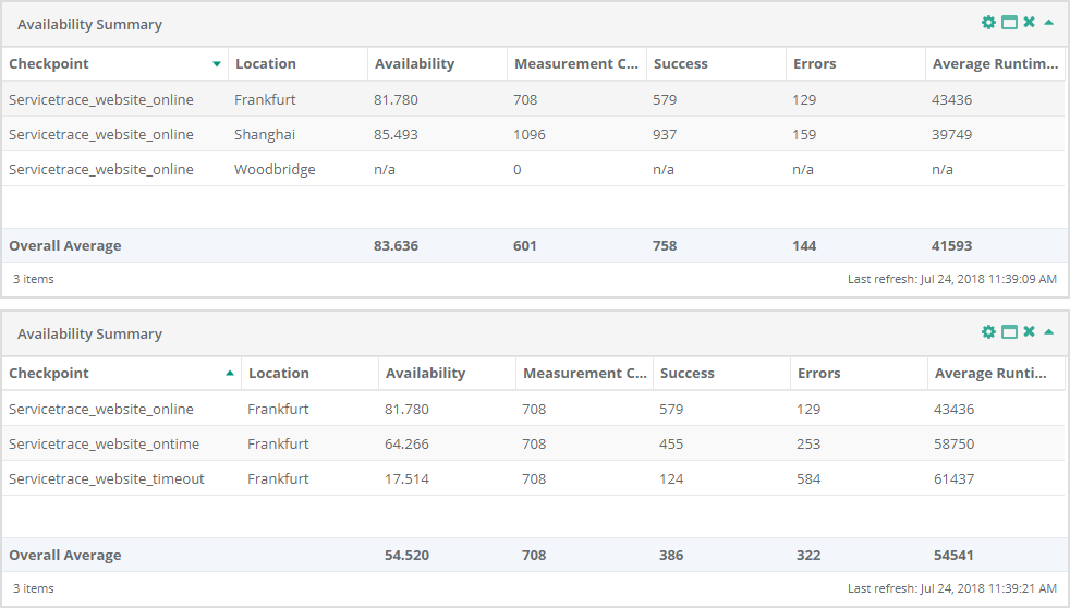
If you want to save such an adjustment permanently, please use the Save button in the Report Properties.
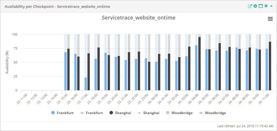
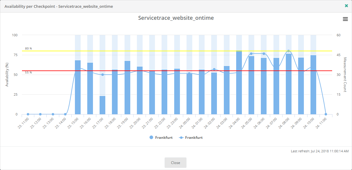
Availability per Checkpoint
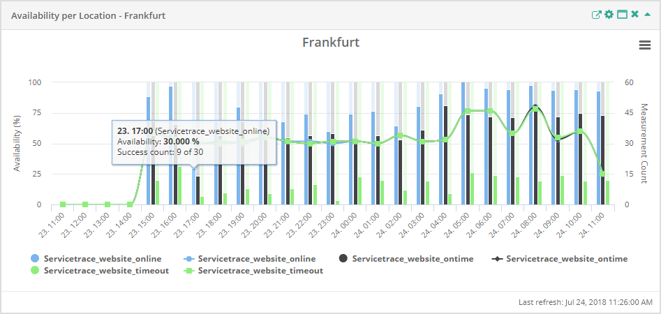
Availability is shown in graph form in the "Availability per Checkpoint" widget. All the time specifications relate to the time zone of the user who is logged in on the Central Server system. Read more about this here.

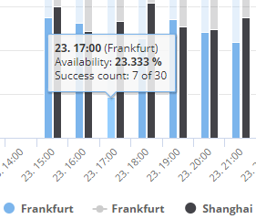
In addition to showing availability, the chart indicates the number of measurements which were used to determine that availability. The number of measurements is overlaid as a line graph with the relevant values evident from the y-axis on the right. This line graph is a quick visual way to capture the number of measurements. The number of measurements can also be found in the tool-tip for a bar within the bar graph.
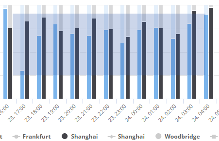
The graph is divided into different size intervals depending on the period under consideration. For each interval, a bar graph shows how high availability was in the individual Locations. Each Location is allocated its own color for this, with a key underneath the graph displaying their association. Locations can also be switched on and off in the key. If you click on a Location, its bars are removed from the display. In this way, the space available on the graph can be used as required.
If the bar shown has a transparent section, then availability did not reach 100% during the corresponding interval. The transparent section represents the percentage of non-availability. If there is no bar at all for a Location during an interval, either transparent or fully colored, then there is no measurement for this interval. Placing the mouse on the bar allows the exact values to be read in a tool-tip.
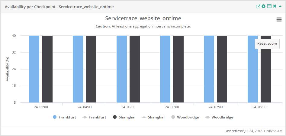
The "Availability per Checkpoint" widget also gives the option of zooming in on the graphs as much as required. Zooming works both on the X and the Y axis here. If you are interested in availability between 80% and 100% during a particular time range, you would highlight the range by placing the mouse at the start of the time range at 80%. Whilst holding down the left mouse button, drag upwards to the 100% mark and to the right up to the end of the time range in question.
As a result, you see an enlarged view of the time range in question. If you would like to change back to the full display, use the "Reset zoom" button for this purpose.
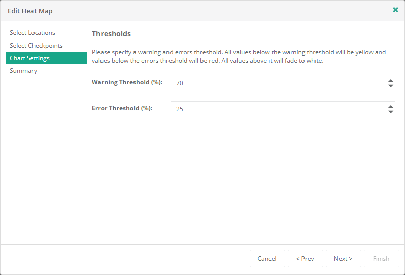
The availability charts show warning and error thresholds, which are user-configurable. These can be used to verify the availability of Customer systems in a visual way. The thresholds appear as a horizontal yellow (for warnings) and red (for errors) line across the chart.
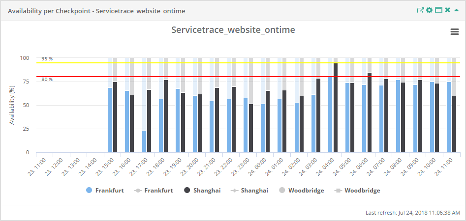
The settings of this widget can be used to specify which checkpoint should be included. It is also possible to define for which Locations the availability of this checkpoint should be listed. This makes it possible to accept Locations added later or to remove Locations that are no longer relevant from the widget.

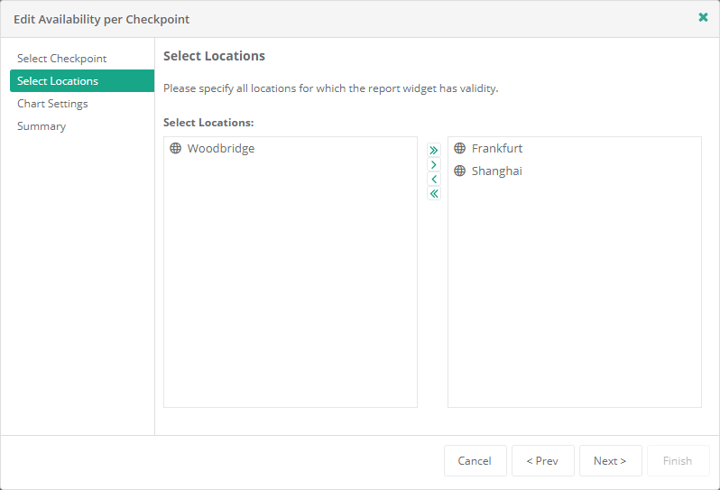
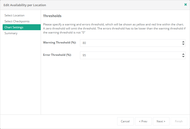
Like the checkpoint and the corresponding Locations, the availability thresholds (warning and error) are user-configurable. The value for the warning threshold must be greater than the error threshold here. A threshold of 0 means that no threshold appears on the chart.

User
This menu item is only available to users with the Service Report Create / Edit
privilege.
If you want to save such an adjustment permanently, please use the Save button in the Report Properties.
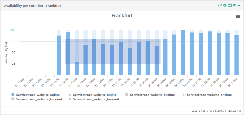
Availability per Location
Availability is shown in graph form in the "Availability per Location" widget. An "Availability per Location" window can also only contain exactly one Location in this case, yet all the checkpoints that were measured from there. All the time specifications relate to the time zone of the user who is logged in on the Central Server system. Read more about this here.
In addition to showing availability, the chart indicates the number of measurements which were used to determine that availability. The number of measurements is overlaid as a line graph with the relevant values evident from the y-axis on the right. This line graph is a quick visual way to capture the number of measurements. The number of measurements can also be found in the tool-tip for a bar within the bar graph.
The graph is divided into different size intervals depending on the period under consideration. For each interval, a bar graph lists how high availability of the individual checkpoint was in the Locations. Each checkpoint is allocated its own color for this, with a key underneath the graph displaying their association. Checkpoints can also be switched on and off in the key. If you click on a checkpoint, its bars are removed from the display. In this way, the space available on the graph can be used as required.
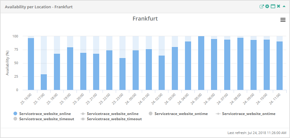
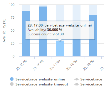
If the bar shown has a transparent section, then availability did not reach 100% during the corresponding interval. The transparent section represents the percentage of non-availability. If there is no bar at all for a checkpoint during an interval, either transparent or fully colored, then there is no measurement for this interval. Placing the mouse on the bar allows the exact values to be read in a tool-tip.
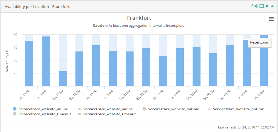
The "Availability per Location" widget also gives the option of zooming in on the graphs as much as required. Zooming works both on the X and the Y axis here. If you are interested in availability between 80% and 100% during a particular time range, you would highlight the range by placing the mouse at the start of the time range at 80%. Whilst holding down the left mouse button, drag upwards to the 100% mark and to the right up to the end of the time range in question.
As a result, you see an enlarged view of the time range in question. If you would like to change back to the full display, use the "Reset zoom" button for this purpose.
The availability charts show warning and error thresholds, which are user-configurable. These can be used to verify the availability of Customer systems in a visual way. The thresholds appear as a horizontal yellow (for warnings) or red (for errors) line across the chart.
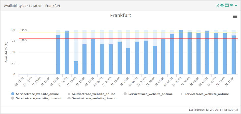
Like the Location and checkpoints, the availability thresholds (warning and error) are user-configurable. The value for the warning threshold must be greater than the error threshold here. A threshold of 0 means that no threshold appears on the chart.
The settings of this widget can be used to specify which Locations should be included. It is also possible to define for which checkpoints measured in this Location the availability should be listed. This makes it possible to accept checkpoints added later or to remove checkpoints that are no longer relevant from the widget.
User
This menu item is only available to users with the Service Report Create / Edit
privilege.
To save the adjustments permanently, please use the Save button in the Report Properties.
Availability Heat Map
The "Availability Heat Map" widget is a graphical overview for fast comprehension of the availability of checkpoints in different Locations. The fields indicating the availability of a checkpoint in a specific Location are color-coded. The less available the checkpoint is, the more intense the color of the field (yellow for warning, red for error). For example, an availability of 100% appears white, an availability of 85% and below shows as yellow, and an availability of 75% and below will appear dark red. The values between the warning or error thresholds appear in graduated shades between the relevant colors. A scale on the right side of the widget shows how the colors relate to the values.
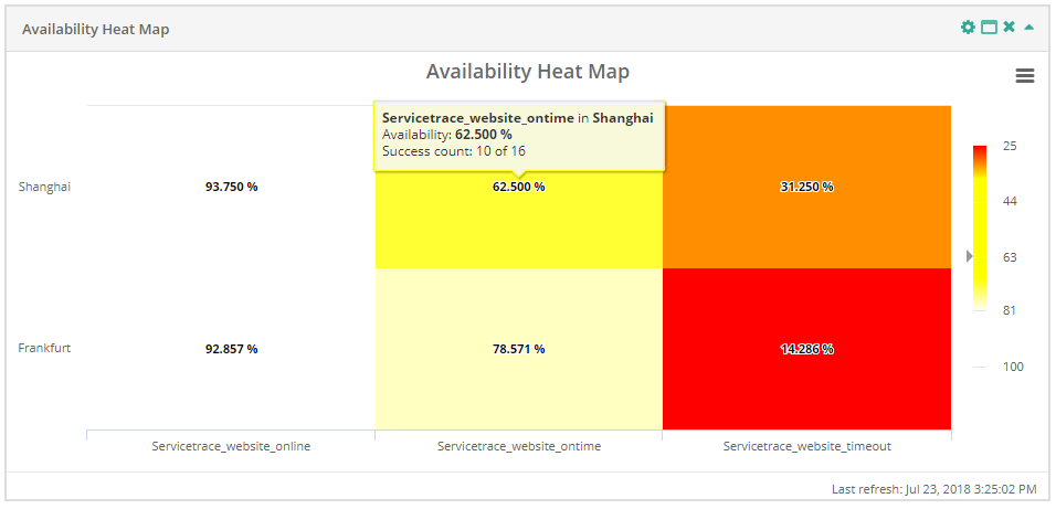
The Availability Heat Map offers a drill-down. A user is able to see a detailed Availability per Checkpoint chart, which leads to the availability shown in the heat map. The drill-down will be shown in an overlay window.
The settings of this widget are used to define from which Locations the measured data is shown. You can also decide for which checkpoints the availability values of these Locations should be included in the Heat Map.


Like the Locations and checkpoints, the warning and error thresholds for the Availability Heat Map are user-configurable. The value for the warning threshold must be greater than the error threshold here. A warning threshold of 0 means that no warning threshold appears on the chart.
User
This menu item is only available to users with the Service Report Create / Edit
privilege.
If you want to save such an adjustment permanently, please use the Save button in the Report Properties.
Response Time Summary
The "Response Time Summary" widget is a list in table form of the response times measured. To determine a response time, timers are set up in the Workflows. The name of the timer is given first accordingly. As measurements may have been taken from different Locations, the Location is also specified. After that, the number of measurements carried out is specified along with the minimum, maximum, and average response time values calculated from the measurements. The last row Overall Average shows the arithmetic average of all values shown in the respective column of the widget.
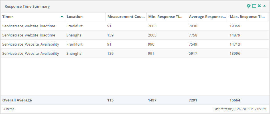
You can also hide the individual columns as required. As an option, you can still show to which System and which Application from the Master Data the timer belongs.

The settings of this widget are used to define from which Locations the measured data is listed. You can also determine for which timers the response times from these Locations should be included in the table.
User
This menu item is only available to users with the Service Report Create / Edit
privilege.
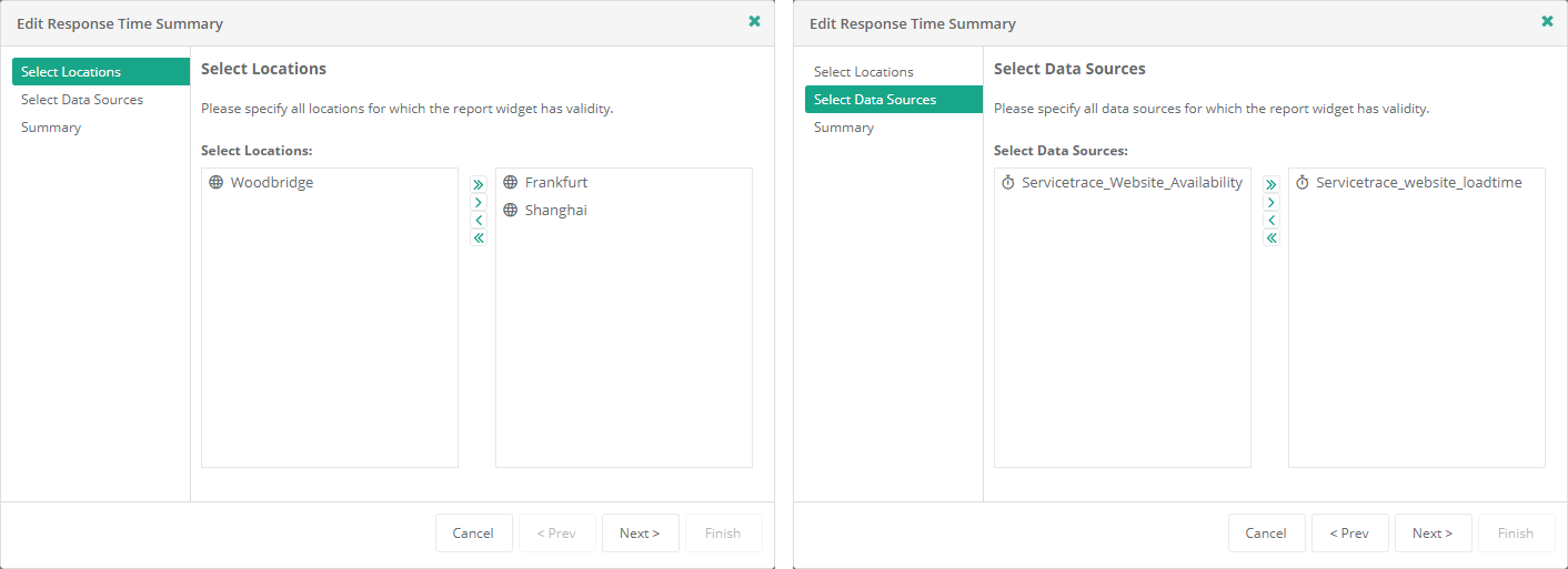
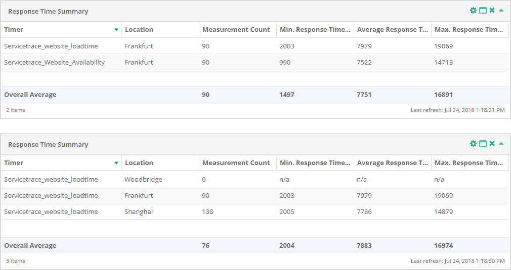
It is therefore possible to either display all the information in one window, or to pool all the timers for one Location or all the Locations for one timer in a single window.
Response Time per Location
Response times measured are displayed in graph form in the "Response Time per Location" widget. A "Response Time per Location" window can also only contain exactly one Location in this case, yet all the timers that were measured from there. All the time specifications relate to the time zone of the user who is logged in on the Central Server system. Read more about this here.

On the graph, the individual measurements are connected in a continuous line. This makes it easy for you to see the progress of the response times. Each timer is allocated its own color for this, with a key underneath the graph displaying their association. Timers can also be switched on and off in the key. If you click on a timer, its line is removed from the display. In this way, the space available on the graph can be used as requir ed. The range of values for the visible timers is automatically adjusted to the value on the Y axis.
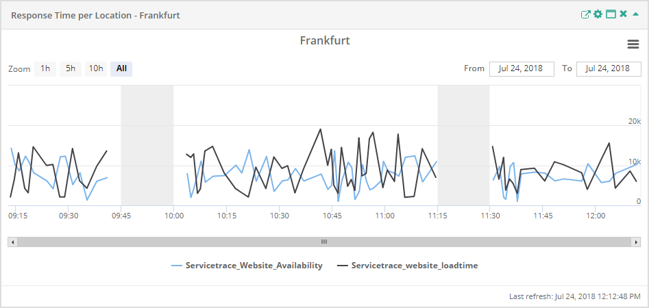
If a section is grayed out on the graph, this shows that the corresponding range is not being evaluated. This is attributable to the Service Times, Down Times, Holidays, and Excluded Measurements that come from the Service underlying the report. If you want to find out about these Service parameters then please look in the report's calendar and from there select the Location that matches the widget. If there is no line at all for a timer, then there are no measurements for the period under consideration.
Placing the mouse on the line allows you to read the exact current measurements in a tooltip.
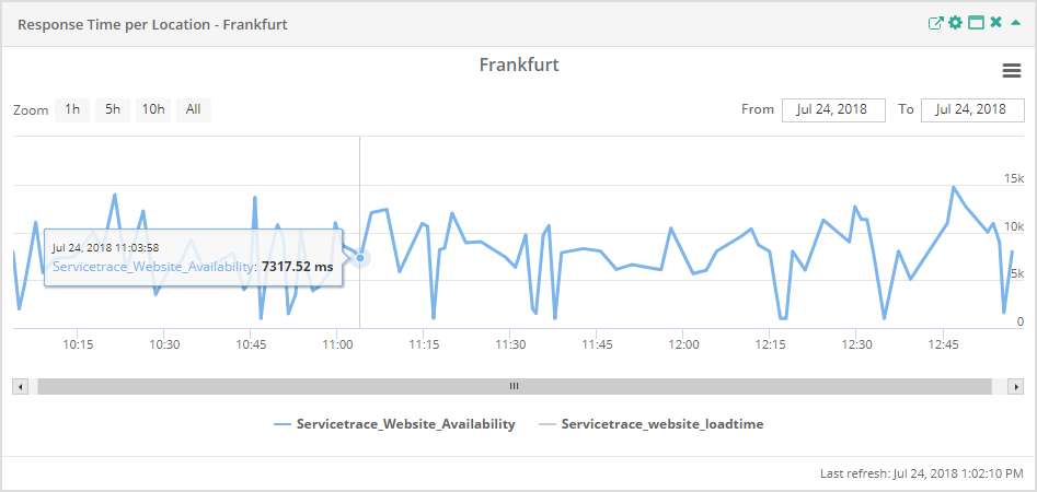
You can also zoom in on the graphs in the "Response Time per Location" window. Zooming only works here on the X axis. If you are interested in the response times during a particular time range, you would highlight these by placing the mouse at the start of the time range. Whilst holding down the left button, drag the mouse to the right to the end of the time range in question. Alternatively you can also use the zoom level suggested at the upper left in the widget.
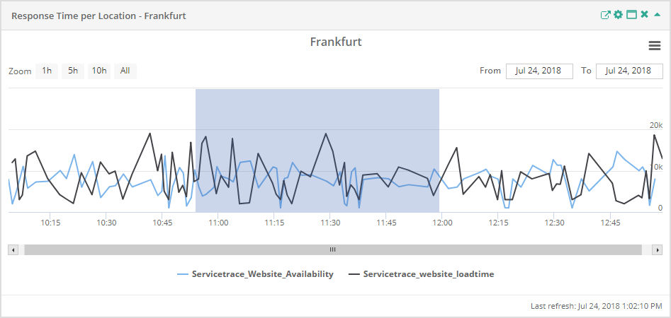
As a result, you see an enlarged view of the time range in question. If the graph is in a zoomed view, you can also move the visible section to an earlier or later point in time using a scroll bar. If you would like to change back to the full display, use the "All" button at the upper left for this purpose.

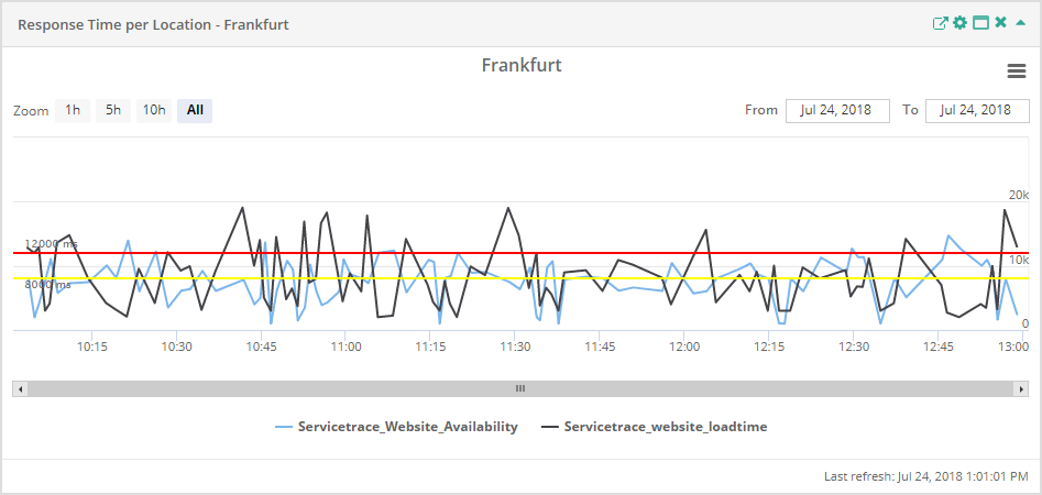
Like the availability charts, it is possible to set and show any threshold for the response time charts. This can be used to verify the response time for Customer systems in a visual way. The threshold appears as a horizontal red line across the graph and indicates to the user the threshold that has been set. It is also possible to switch the scale for the y-axis between linear and logarithmic. A logarithmic y-axis has advantages when analyzing response time values that vary greatly.
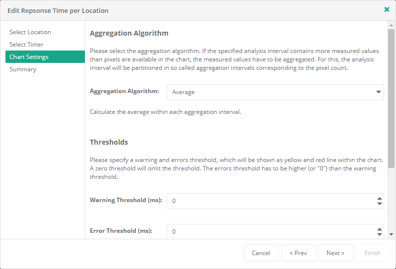
Another special feature of the response time charts is measurement aggregation on the server side. When presenting many measurements on a single monitor, there are inevitably problems with showing a set of values using a finite number of pixels. If the number of measurements is greater than the number of pixels available in the chart, it is necessary to aggregate measurements. Depending on the number of measurements, this can be a very time-consuming and costly operation on the client side (browser). As an example, let's assume 1,000,000 measurements are to be shown using 800 pixels. To boost performance, the appropriate web Service carries out any aggregation that is necessary on the web server side. As a result, only as many measurement values need to be transmitted as there are pixels available for the relevant chart. Aggregation provides a calculated value that depends on the method applied. Servicetrace Reporting allows the user to specify an aggregation algorithm that is suitable for their respective use case. The following algorithms are available:
| Average (mean) | The mean of the values contained within the relevant aggregation interval |
| Maximum | Uses the highest value from within the relevant aggregation interval |
| Minimum | Uses the lowest value from within the relevant aggregation interval |
| Open | Uses the first value from the relevant aggregation interval |
| Close | Uses the last value from the relevant aggregation interval |
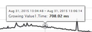
If at least one measurement value in a series has been aggregated, a notification is shown below the title of the response time chart. This information includes the aggregation algorithm that was used.

In the case of an aggregated measurement, the tool-tip shows a time range and not a particular point in time.

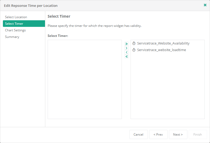
The settings of this widget can be used to specify which Locations should be included. You can also define here for which timers measured in this Location the response times should be shown. You can use this to add timers later or to remove timers that are no longer relevant from the widget.

Like the Location and checkpoints, the aggregation algorithm, response time thresholds (warning and error), and scale for the y-axis are user-configurable. A threshold of 0 means that no threshold appears on the chart.
User
This menu item is only available to users with the Service Report Create / Edit
privilege.
To save such adjustments permanently, please use the Save button in the Report Properties.
Aggregated Response Time per Location
Response times measured are displayed in graph form in the "Aggregated Response Time per Location" widget. A "Aggregated Response Time per Location" window can only contain exactly one Location in this case, yet all the timers that were measured from that location. All the time specifications relate to the time zone of the user who is logged in on the Central Server system. Read more about this here.
In addition to the chart, the widget also contains an overview table with all the values displayed in the chart.
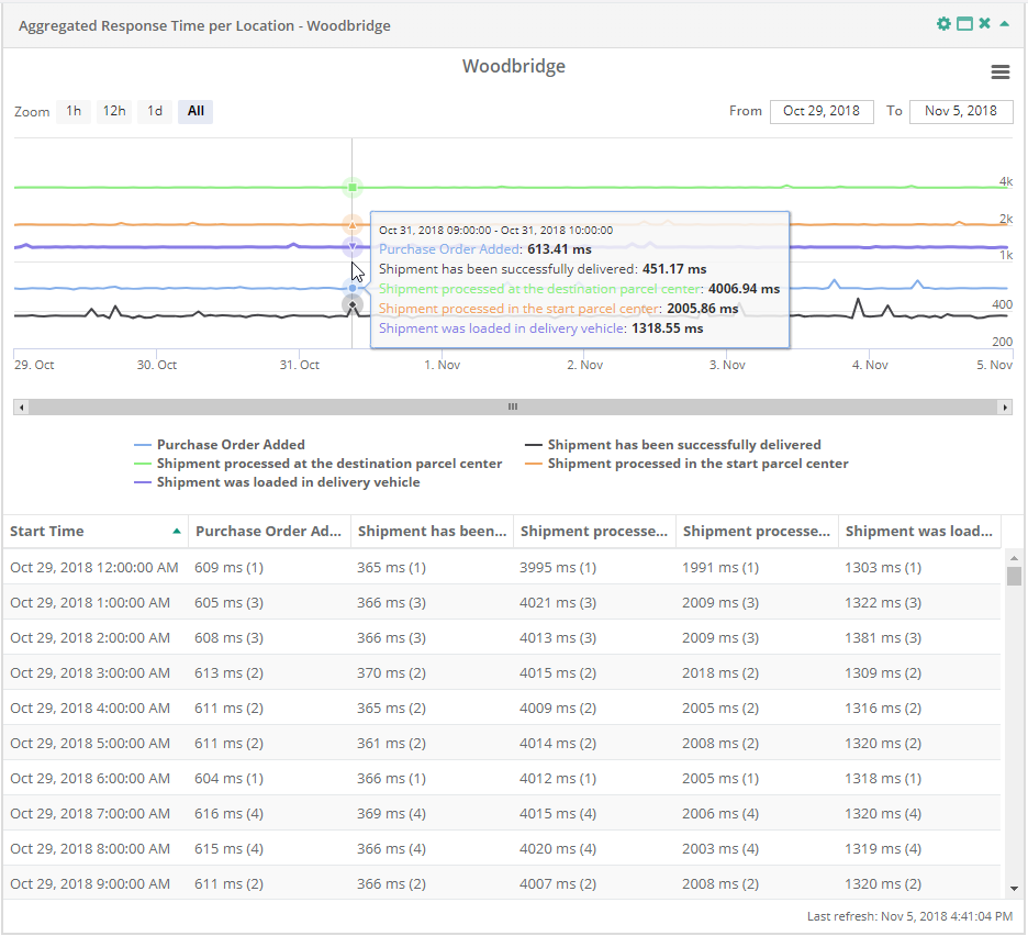
On the graph, the individual measurements are connected in a continuous line. This makes it easy for you to see the progress of the response times. Each timer is allocated its own color for this, with a key underneath the graph displaying their association. Timers can also be switched on and off in the key. If you click on a timer, its line is removed from the display. In this way, the space available on the graph can be used as required. The range of values for the visible timers is automatically adjusted to the value on the Y axis.
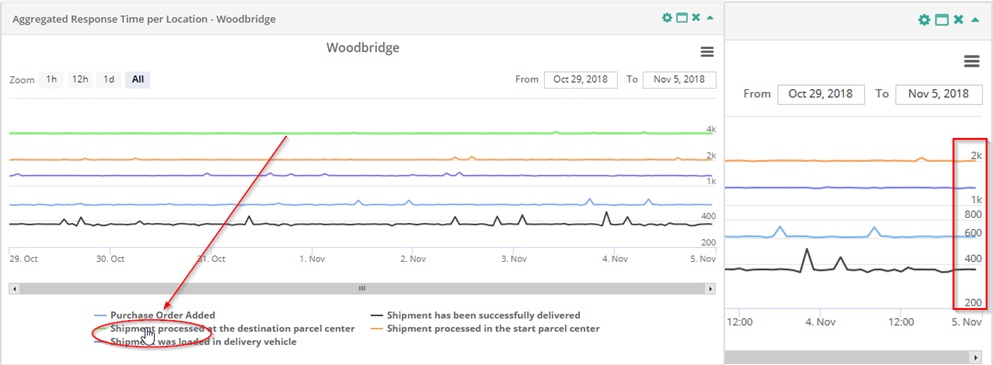
If there is a gap in a section on the graph, it shows that the corresponding range is not being evaluated. You will find the gap also in the table below. This is attributable to the Service Times, Down Times, Holidays, and Excluded Measurements that come from the Service underlying the report. If you want to find out about these Service parameters then please look in the report's calendar and from there select the Location that matches the widget. If there is no line at all for a timer, then there are no measurements for the period under consideration.

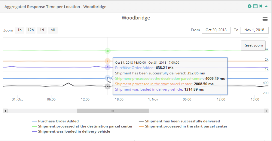
Placing the mouse on the line allows you to read the exact current measurements in a tooltip.

You can also zoom in on the graphs in the "Aggregated Response Time per Location" window. Zooming only works here on the X axis. If you are interested in the response times during a particular time range, you would highlight these by placing the mouse at the start of the time range. Whilst holding down the left button, drag the mouse to the right to the end of the time range in question. Alternatively you can also use the zoom level suggested at the upper left in the widget.
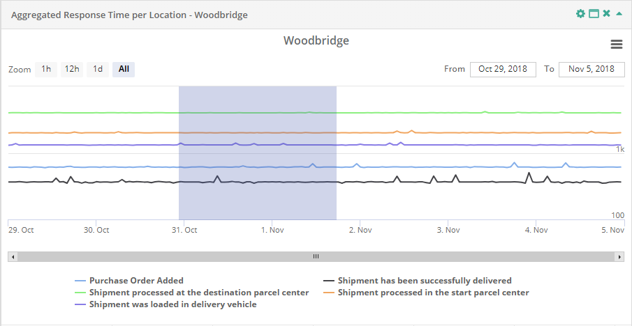
As a result, you see an enlarged view of the time range in question. If the graph is in a zoomed view, you can also move the visible section to an earlier or later point in time using a scroll bar. If you would like to change back to the full display, use the "All" button at the upper left or the "Reset zoom" button at the upper right for this purpose.
Like the availability charts, it is possible to set and show any threshold for the response time charts. This can be used to verify the response time for Customer systems in a visual way. The threshold appears as a horizontal red line across the graph and indicates to the user the threshold that has been set. It is also possible to switch the scale for the y-axis between linear and logarithmic. A logarithmic y-axis has advantages when analyzing response time values that vary greatly.

Another special feature of the aggregated response time charts is measurement aggregation on the server side. When presenting many measurements on a single monitor, there are inevitably problems with showing a set of values using a finite number of pixels. If the number of measurements is greater than the number of pixels available in the chart, it is necessary to aggregate measurements. Depending on the number of measurements, this can be a very time-consuming and costly operation on the client side (browser). As an example, let's assume 1,000,000 measurements are to be shown using 800 pixels. To boost performance, the appropriate web Service carries out any aggregation that is necessary on the web server side. As a result, only as many measurement values need to be transmitted as there are pixels available for the relevant chart. Aggregation provides a calculated value that depends on the method applied. Servicetrace Reporting allows the user to specify an aggregation algorithm that is suitable for their respective use case. The following algorithms are available:
| Average (mean) | The mean of the values contained within the relevant aggregation interval |
| Maximum | Uses the highest value from within the relevant aggregation interval |
| Minimum | Uses the lowest value from within the relevant aggregation interval |
| Open | Uses the first value from the relevant aggregation interval |
| Close | Uses the last value from the relevant aggregation interval |
In the case of an aggregated measurement, the tool-tip shows a time range and not a particular point in time.
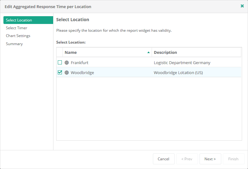
The settings of this widget can be used to specify which Locations should be included. You can also define here for which timers measured in this Location the response times should be shown. You can use this to add timers later or to remove timers that are no longer relevant from the widget.
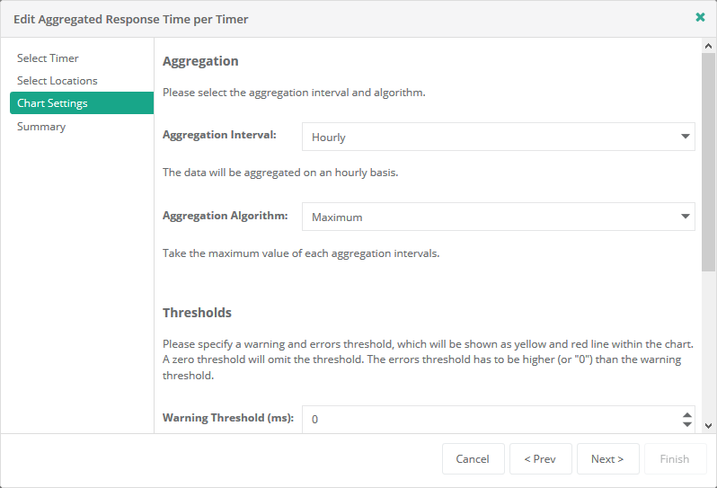
Like the Location and Timer, the aggregation algorithm, response time thresholds (warning and error), and scale for the y-axis are user-configurable. In addition to that you have the setting Aggregation Interval, where you can change the interval from Hourly to Daily. This means the data will be aggregated on an hourly or daily basis. A threshold of 0 means that no threshold appears on the chart.

User
This menu item is only available to users with the Service Report Create / Edit
privilege.
To save such adjustments permanently, please use the Save button in the Report Properties.
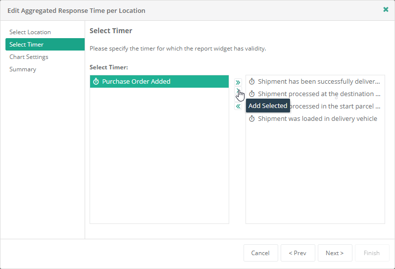
Response Time per Timer
Response times measured are displayed in graph form in the "Response Time per Timer" widget. A "Response Time per Timer" window can also only contain exactly one timer in this case, yet all the Locations where this was measured. All the time specifications relate to the time zone of the user who is logged in on the Central Server system. Read more about this here.
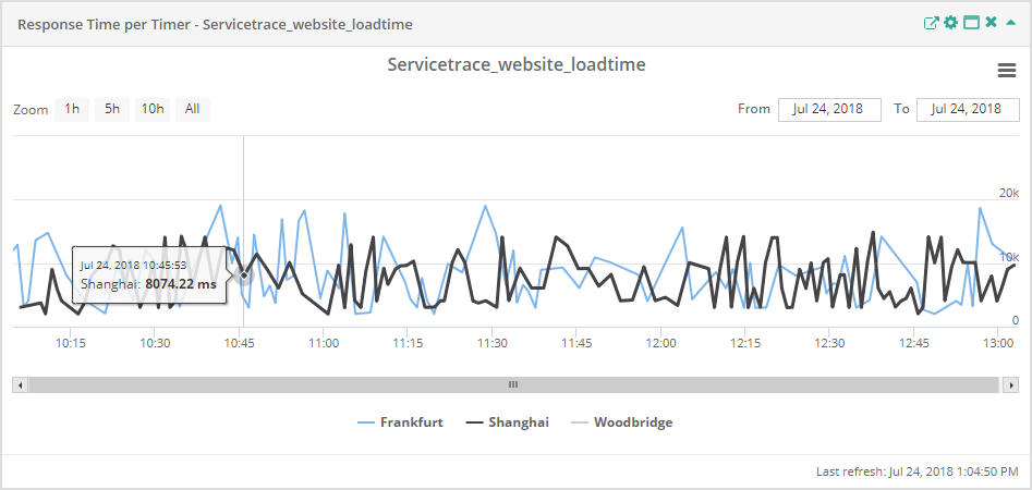
On the graph, the individual measurements are connected in a continuous line to make it easy for you to see the progress of the response times. Each Location is allocated its own color for this, with a key underneath the graph displaying their association. Locations can also be switched on and off in the key. If you click on a Location, its line is removed from the display. In this way, the space available on the graph can be used as required. The range of values on the Y axis is automatically adjusted to the values of the visible timers.
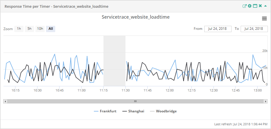
If the graph contains grayed out areas, this means that measurements are not evaluated here. This is attributable to the Service Times, Down Times, Holidays, and Excluded Measurements that come from the Service underlying the report.
In this widget, it may be the case that measurements are nevertheless shown as a line in a grayed out area. This then means that there was no Service Time at this time in one of the Locations, but that the measurements displayed inside the grayed out area come from a Location that had a Service Time at this time. In the report's calendarp you will find detailed information about this Service Time.
If there is no line at all for a timer, then there are no measurements for the period under consideration.
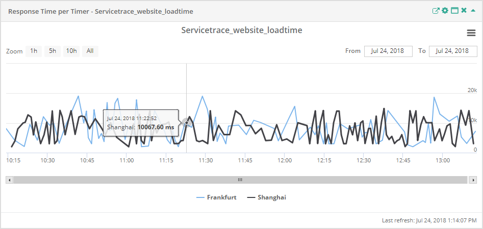
Placing the mouse on the line allows you to read the exact current measurements in a tool-tip.
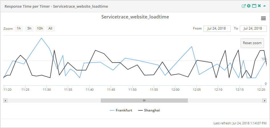
You can also zoom in on the graphs in the "Response Time per Timer" widget. Zooming only works on the X axis here. If you are interested in the response times during a particular time range, highlight these by placing the mouse at the start of the time range. Whilst holding down the left button, drag the mouse to the right to the end of the time range in question. Alternatively you can use the zoom level suggested at the upper left in the widget.
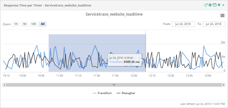
As a result, you see an enlarged view of the time range in question. If the graph is in a zoomed view, you can also move the visible section to an earlier or later point in time using a scroll bar. If you would like to change back to the full display, use the "All" button at the upper left for this purpose.
Like the availability charts, it is possible to set and show any threshold for the response time charts. This can be used to verify the response time for Customer systems in a visual way. The threshold appears as a horizontal red line across the graph and indicates to the user the threshold that has been set. It is also possible to switch the scale for the y-axis between linear and logarithmic. A logarithmic y-axis has advantages when analyzing response time values that vary greatly.
Another special feature of the response time charts is measurement aggregation on the server side. When presenting many measurements on a single monitor, there are inevitably problems with showing a set of values using a finite number of pixels. If the number of measurements is greater than the number of pixels available in the chart, it is necessary to aggregate measurements. Depending on the number of measurements, this can be a very time-consuming and costly operation on the client side (browser). As an example, let's assume 1,000,000 measurements are to be shown using 800 pixels. To boost performance, the appropriate web Service carries out any aggregation that is necessary on the web server side. As a result, only as many measurement values need to be transmitted as there are pixels available for the relevant graph. Aggregation provides a calculated value that depends on the method applied. Servicetrace Reporting allows the user to specify an aggregation algorithm that is suitable for their respective use case. The following algorithms are available:
| Average (mean) | The mean of the values contained within the relevant aggregation interval |
| Maximum | Uses the highest value from within the relevant aggregation interval |
| Minimum | Uses the lowest value from within the relevant aggregation interval |
| Open | Uses the first value from the relevant aggregation interval |
| Close | Uses the last value from the relevant aggregation interval |
If at least one measurement value in a series has been aggregated, a notification is shown below the title of the response time chart. This information includes the aggregation algorithm that was used.
In the case of an aggregated measurement, the tool-tip shows a time range and not a particular point in time.
The settings of this widget can be used to specify which timers should be included. You also define for which Locations the response times of the timer should be shown. You can thus accept Locations added later or remove Locations that are no longer relevant from the widget.
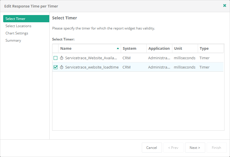

As well as configuring the Checkpoint and Locations, the user is able to freely configure the aggregation algorithm, the response time threshold, and the scale for the y-axis. A threshold of 0 means that no threshold appears on the chart.

User
This menu item is only available to users with the Service Report Create / Edit
privilege.
To save such adjustments permanently, please use the Save button in the Report Properties.
Aggregated Response Time per Timer
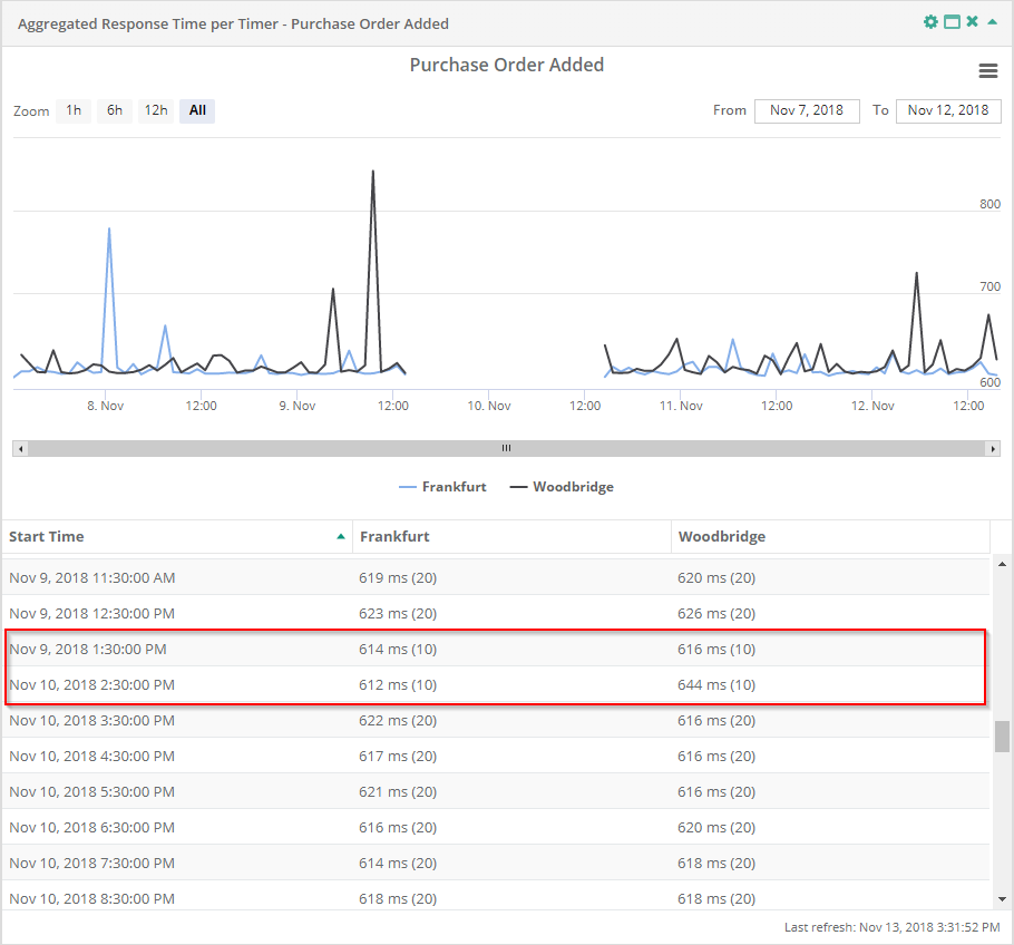
Aggregated response times measured are displayed in graph form in the "Aggregated Response Time per Timer" widget. A "Aggregated Response Time per Timer" window can also only contain exactly one timer in this case, yet all the Locations where this was measured. All the time specifications relate to the time zone of the user who is logged in on the Central Server system. Read more about this here.
In addition to the chart, the widget also contains an overview table with all the values displayed in the chart.

On the graph, the individual measurements are connected in a continuous line to make it easy for you to see the progress of the response times. Each Location is allocated its own color for this, with a key underneath the graph displaying their association. Locations can also be switched on and off in the key. If you click on a Location, its line is removed from the display. In this way, the space available on the graph can be used as required. The range of values on the Y axis is automatically adjusted to the values of the visible timers.
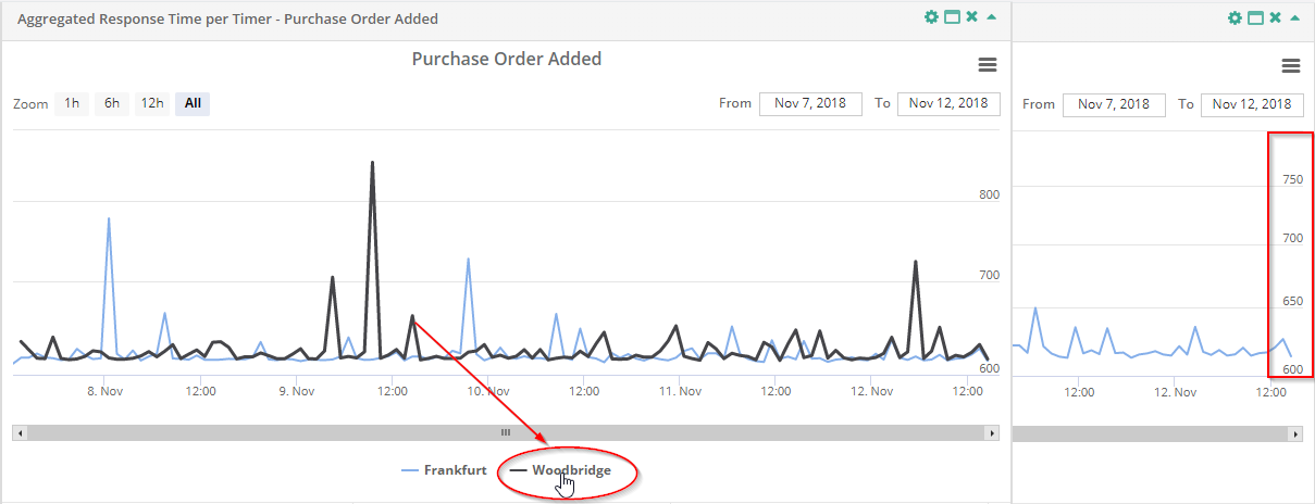
If there is a gap in a section on the graph, it shows that the corresponding range is not being evaluated. You will find the gap also in the table below. This is attributable to the Service Times, Down Times, Holidays, and Excluded Measurements that come from the Service underlying the report.
In this widget, it may be the case that measurements are nevertheless shown as a line inside the gap. This means that there was no Service Time at this time in one of the Locations and the measurements displayed inside the gap comes from a Location that had a Service Time at this time. In the report's calendar you will find detailed information about this Service Time.
If there is no line at all for a timer, then there are no measurements for the period under consideration.
Placing the mouse on the line allows you to read the exact current measurements in a tool-tip.
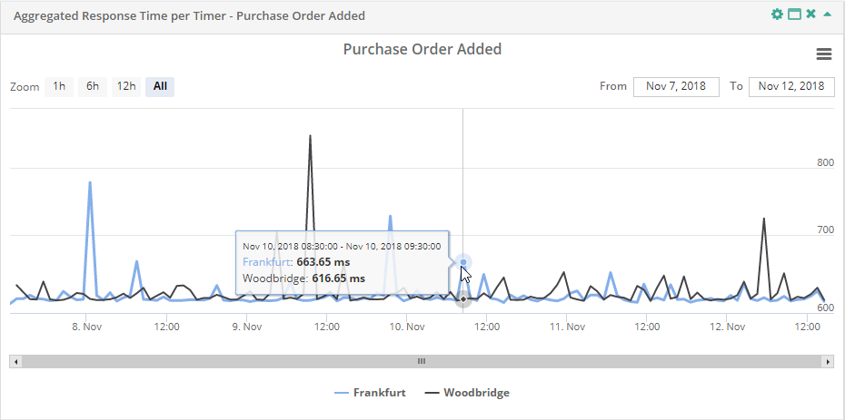
You can also zoom in on the graphs in the "Aggregated Response Time per Timer" widget. Zooming only works on the X axis here. If you are interested in the response times during a particular time range, highlight these by placing the mouse at the start of the time range. Whilst holding down the left button, drag the mouse to the right to the end of the time range in question. Alternatively you can use the zoom level suggested at the upper left in the widget.

As a result, you see an enlarged view of the time range in question. If the graph is in a zoomed view, you can also move the visible section to an earlier or later point in time using a scroll bar. If you would like to change back to the full display, use the "All" button at the upper left or the "Reset zoom" button at the upper right for this purpose.

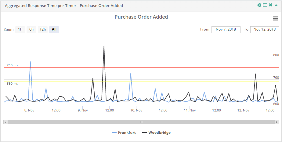
Like the availability charts, it is possible to set and show any threshold for the response time charts. This can be used to verify the response time for Customer systems in a visual way. The threshold appears as a horizontal red line across the graph and indicates to the user the threshold that has been set. It is also possible to switch the scale for the y-axis between linear and logarithmic. A logarithmic y-axis has advantages when analyzing response time values that vary greatly.
Another special feature of the response time charts is measurement aggregation on the server side. When presenting many measurements on a single monitor, there are inevitably problems with showing a set of values using a finite number of pixels. If the number of measurements is greater than the number of pixels available in the chart, it is necessary to aggregate measurements. Depending on the number of measurements, this can be a very time-consuming and costly operation on the client side (browser). As an example, let's assume 1,000,000 measurements are to be shown using 800 pixels. To boost performance, the appropriate web Service carries out any aggregation that is necessary on the web server side. As a result, only as many measurement values need to be transmitted as there are pixels available for the relevant graph. Aggregation provides a calculated value that depends on the method applied. Servicetrace Reporting allows the user to specify an aggregation algorithm that is suitable for their respective use case. The following algorithms are available:
| Average (mean) | The mean of the values contained within the relevant aggregation interval |
| Maximum | Uses the highest value from within the relevant aggregation interval |
| Minimum | Uses the lowest value from within the relevant aggregation interval |
| Open | Uses the first value from the relevant aggregation interval |
| Close | Uses the last value from the relevant aggregation interval |
In the case of an aggregated measurement, the tool-tip shows a time range and not a particular point in time.
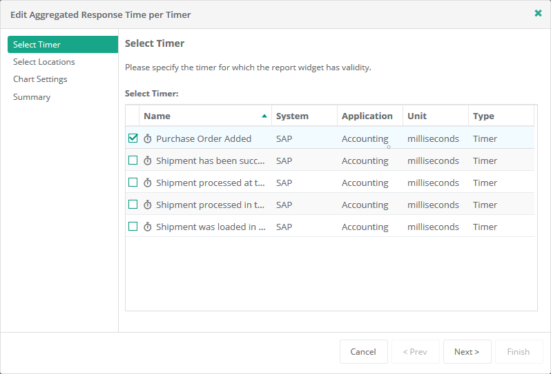
The settings of this widget can be used to specify which timers should be included. You also define for which Locations the response times of the timer should be shown. You can thus accept Locations added later or remove Locations that are no longer relevant from the widget.

As well as configuring the Timer and Locations, you are able to freely configure the aggregation algorithm, the response time threshold, and the scale for the y-axis. In addition to that the setting Aggregation Interval is available. Here you can change the interval from Hourly to Daily. A threshold of 0 means that no threshold appears on the chart.
User
This menu item is only available to users with the Service Report Create / Edit
privilege.
To save such adjustments permanently, please use the Save button in the Report Properties.
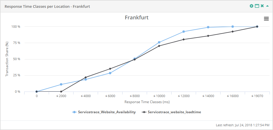
Response Time Classes per Location
Response times measured are displayed in graph form in the "Response Time Classes per Location" widget. A "Response Time Classes per Location" window can also only contain exactly one Location in this case, yet all the timers that were measured from there. In contrast to then"Response Time per Location" display, the timers are not shown on a time axis here but according to their distribution in percentage terms. That means the X axis shows the response time increasing to the right, and the Y axis the percentage increasing upwards. From this graph you can see how many measurements for a particular action resulted in less than X milliseconds.
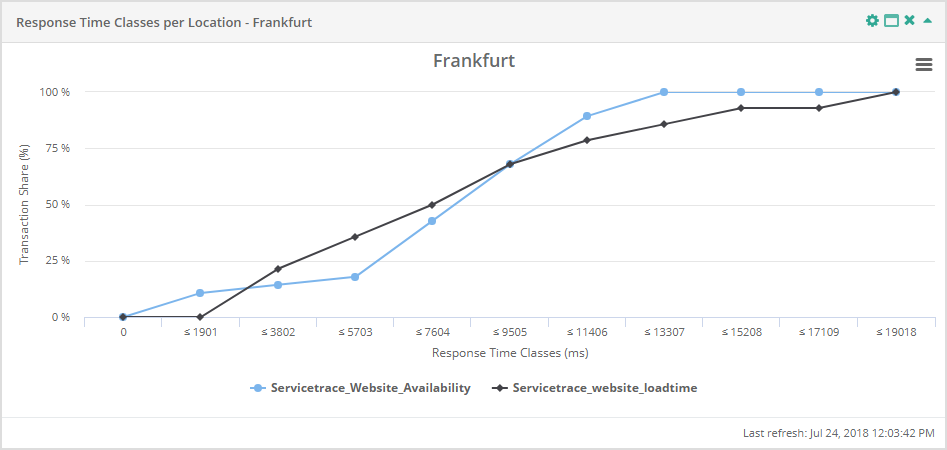
This graphs shows whether a transaction varies widely in its response times or whether it responds very uniformly. Slowly rising curves mean widely varying response times. Quickly rising curves, which soon approach the 100% mark, mean very uniform response times. You can thus spot slightly sporadic "rogue results" in a high response time range: this is the case if the curve quickly approaches the 95%+ mark, but 100% of the measurements made were only completed at high response times.
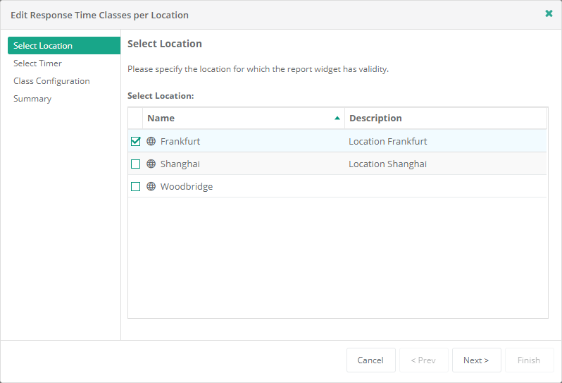
The settings of this widget are used to define which Locations should be included. You can also determine for which timers measured in this Location the response times should be shown. You can use this to add new timers later or to remove timers that are no longer relevant from the widget.

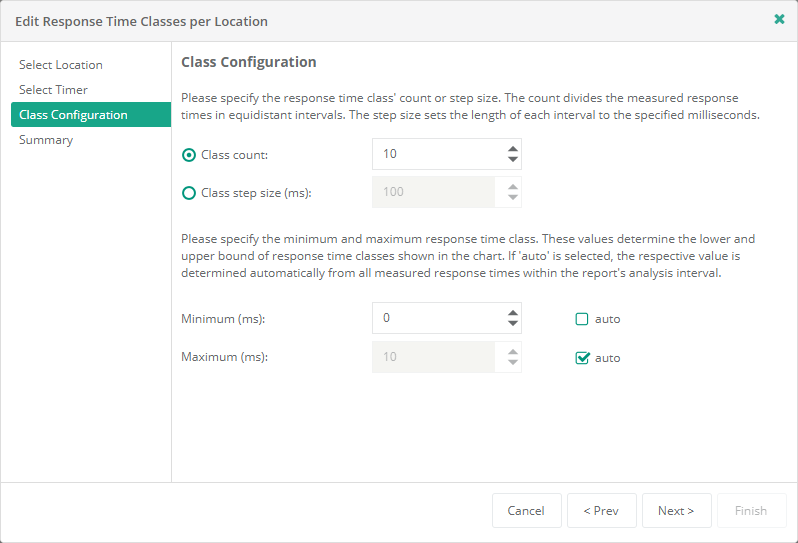
Unlike other "Response Time" graphs, no individual measurement points are specified here. When this widget is set up (or later using the settings), you define how many sections the graph should be divided into. You can specify a set number of areas or an increment in milliseconds. In addition, you can specify a minimum and maximum response time so that the graph only starts or finishes at this value. You can allow the start and finish to be determined automatically depending on the measurement data available during the report's period under consideration. This results in a particular number of individual values that are displayed on the "Response Time Classes" graph. Either increase the "class count" or reduce the "step size" in order to display more individual values on the graph, thus giving a finer gradation.
User
Adjustments made using the Settings menu item are only available to users with the Service
Report Create / Edit privilege.
Each timer included on the graph is allocated its own color, with a key underneath the graph displaying their association. Timers can also be switched on and off in the key. If you click on a timer, its line is removed from the display. In this way, the space available on the graph can be used as required.
For reasons of comparability, all graphs for the same response times show a value of the measurements completed by that time in percent. To put it another way, the percentage for a particular response time on the graph tells you that this proportion of the measurements carried out were at least this fast, or even faster.
Place the mouse on a line to see exactly what percentage of the measurements made was completed by this response time value.
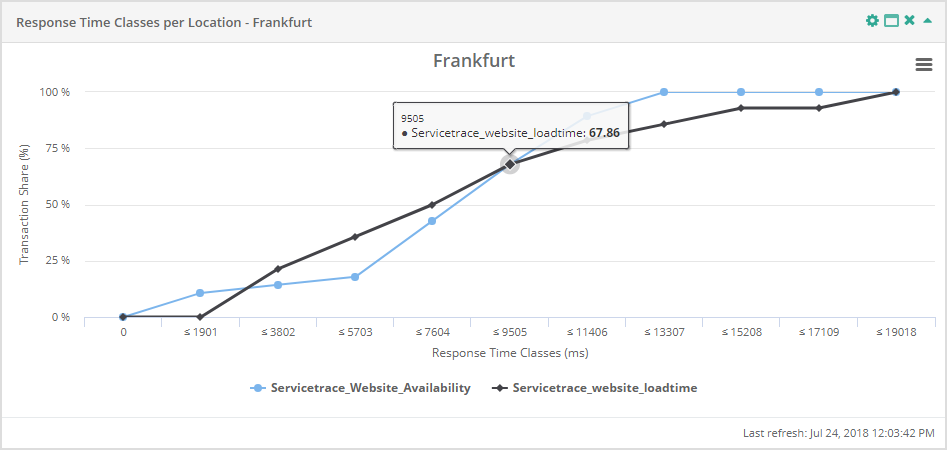
In this example, 97.8% of the measurements made on the "Ramp TestpPattern" timer in New York as a Location were completed after 971 milliseconds or faster.
You can also zoom in on the graphs in the "Response Time Classes per Location" widget. Zooming works both on the X and the Y axis here. If you are interested in the percentage distribution of the response times between zero and two seconds and the area between 70% and 100% of the measurements made, you would highlight the range by placing the mouse at the start of the time range at 80%. Whilst holding down the left mouse button, drag upwards to the 100% mark and to the right up to the end of the time range in question.
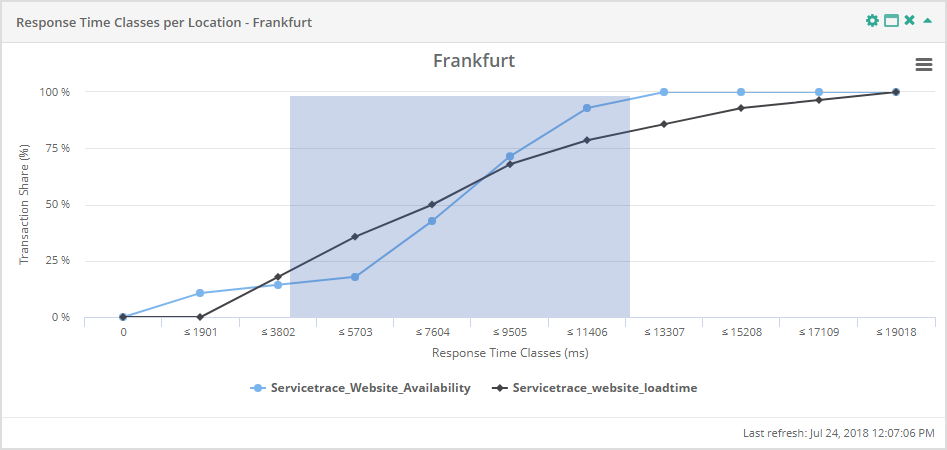
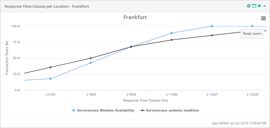
As a result, you see an enlarged view of the time range in question. The number of values contained there does not change by zooming. This is only possible by using class configuration in the settings. If you would like to change back to the full display, use the "Reset zoom" button for this purpose.
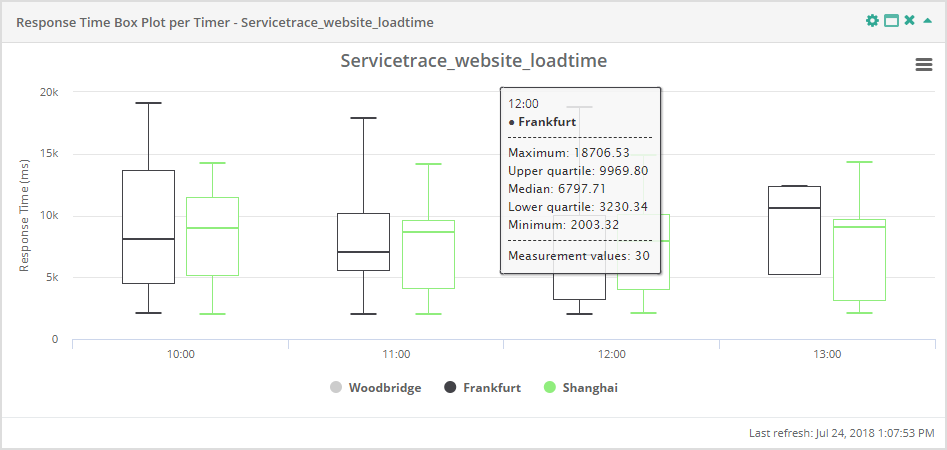
Response Time per Timer Boxplot
The box plot widget shows a graphical representation of the response times of one Timer for several Locations aggregated for the specified
time interval using statistical quartiles.
You can see the ranges of the Timer values for specific periods at one glance. The length of this periods depends on the selected time
interval. For each period the statistical quartile values of the measurement points are shown for each location separately.
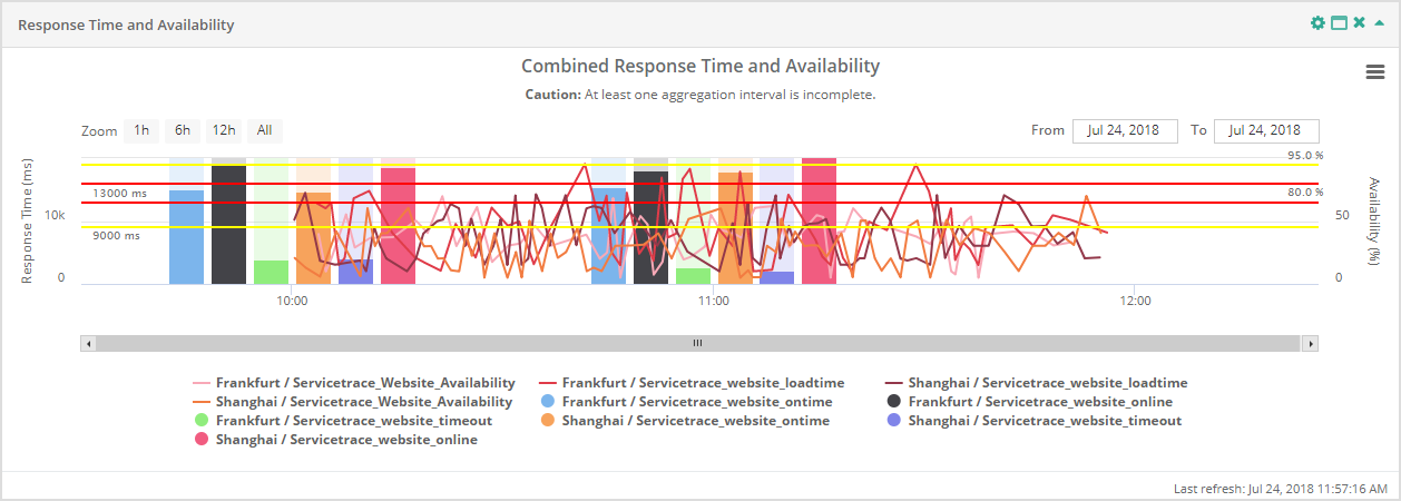
Response Time and Availability
This widget shows an overlay of response time and availability for a combination of Locations and Data Sources.
Service Log
The "Service Log" widget is used to integrate the entries stored in the Service log with the report.
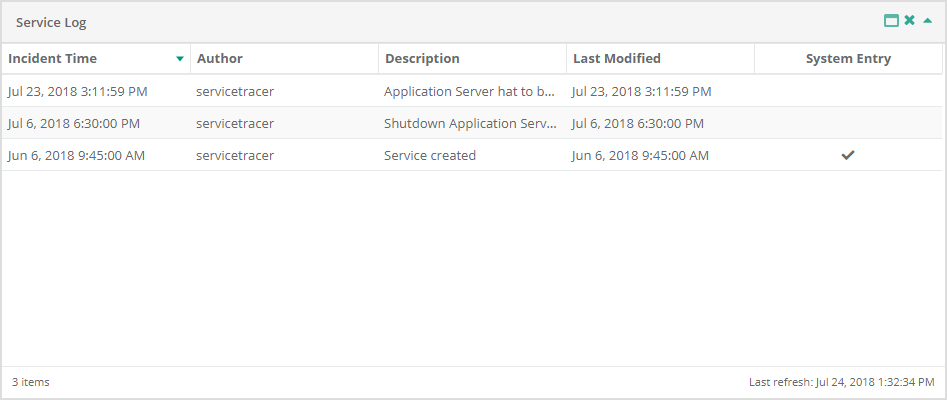
The Service Log is part of the Service underlying the report. It is used to document special incidents and analyses already made. For this purpose, corresponding entries are generated in the Service, each of which relates to a particular point in time. If this point in time lies within the current period under consideration by the report, the corresponding Service Log entry is listed here.
Exporting Graphs
All widgets that contain graphs have an export function. You will find the Chart Context menu at the upper right in the corresponding widgets.

You can export the graph directly as an image in the PNG or JPG formats or also generate a PDF document or vector graphic in the .svg format.
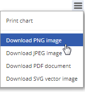
In addition, you can open the graph separately in your browser using "Print Chart". This automatically calls up the "Print" function and you can select a connected printer. Once you have placed or cancelled the print job, the browser automatically returns to the report view.
Time Zones
All the time specifications made in the Service Report relate to the time zone of the user who is logged in on the Central Server system. This applies both to the measurement data shown and to information about Service Times, Down Times or Excluded Measurements.
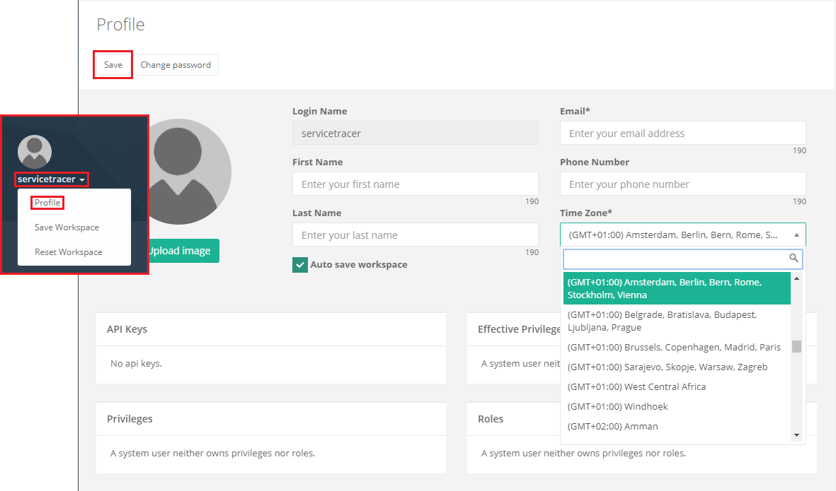
To find out which time zone your user is using, and to change this if necessary, you can click on your user name at the upper left in any of the web apps. The "Profile" option takes you to a summary page of your personal profile settings. Here you can adjust your personal settings, but also those of the time zone used.
This function enables you to conveniently compare measurement data from different Locations within a report, even if these are in different time zones. Caution: If you discuss the evaluation of measurement data with colleagues who work in other time zones, bear in mind that they most likely use their own time zone for display purposes and that the measurement data in the report is shifted accordingly!
If you would like to find out more about the concept of time zones in the Central Server system and how these are shown across the Service, then you will find a detailed description here
Generating Export URLs
This section describes how to address the interface for exporting data from the system. First you need the base URL. The structure is as follows:
<protocol>://<domain:port>/STServices/Reporting/ReportServiceRESTStream.svc |
<base_url>/export/responseTimeCsv? |
This end point supplies data on response times from the system. |
<base_url>/export/resp.availabilityCsv? |
This end point supplies data on availability from the system. |
After the end point, further parameters must be provided in order to specify the data for export more precisely.
start=<startUTC> |
The start time in UTC of the analysis interval for use. The analysis interval is specified by a right-open interval, i.e. the start time is included. Times are entered in ISO 8601 format (yyyy-MM-dd'T'HH:mm:ss.SSSZZ). |
end=<endUTC> |
The end time in UTC of the analysis interval for use. The analysis interval is specified by a right-open interval, i.e. the end time is excluded. Times are entered in ISO 8601 format (yyyy-MM-dd'T'HH:mm:ss.SSSZZ). |
dataSources=<checkpointIDs> |
A comma separated list of Checkpoints for inclusion in the export. The list must not contain any blank spaces. This parameter is optional. If this parameter is not specified in the HTTP request, all Checkpoints from the relevant Service will be used. A section here explains how to obtain these IDs. |
locations=<locationIds> |
A comma separated list of Locations for inclusion in the export. The list must not contain any blank spaces. This parameter is optional. If this parameter is not specified in the HTTP request, all Checkpoints from the relevant Service will be used. A section here explains how to obtain these IDs. |
serviceTimes=<true/false> |
Must contain only "true" or "false" and specifies whether the Service times are to be considered (true) or not (false). |
plannedDownTimes=<true/false> |
Must contain only "true" or "false" and specifies whether the Planned Down Times are to be considered (true) or not (false). |
unplannedDownTimes=<true/false> |
Must contain only "true" or "false" and specifies whether the Unplanned Down Times are to be considered (true) or not (false). |
excludedMeasurements=<true/false> |
Must contain only "true" or "false" and specifies whether excluded measurements are to be considered (true) or not (false). |
holidays=<true/false> |
Must contain only "true" or "false" and specifies whether holidays are to be considered (true) or not (false). |
loginName=<loginName> |
The login name for logging into the web interface and which is assigned to the tenant (Customer). |
password=<password> |
The password that belongs to the login name in the parameter above. Must be in plain text |
How do I obtain the IDs?
The IDs can be found via the web interface. A new "ID" column can be shown for this in the Master Data application.
Export Interface Return
The export interface return value contains the requested data in a CSV-format (separated by "|") in the body of the http response. The format-is as follows:
customer|Service|location|station|datasource|Workflow|date|value|hit
The data in the individual columns are as follows:
| Customer | Name of the relevant Customer (tenant) |
| Service | Name of the relevant Service |
| Location | Name of the relevant Location |
| Station | Name of the relevant Station |
| datasource | Name of the relevant Data Source |
| Workflow | Name of the relevant Workflow |
| date | Time of measurement in ISO 8601 format (yyyy-MM-dd'T'HH:mm:ss.SSSZZ). |
| value | ResponseTimeCsv: answer in milliseconds. AvailabilityCsv: number of seconds from the start of the Workflow to the relevant checkpoint. |
| hit | Indicates whether the checkpoint or response time was reached/achieved (true) or not (false). |